节作者：Jonathon Love

Combining jamovi and R

A huge advantage of jamovi is that it is not only built on top of the R statistical language, it also makes it also very easy to access R from jamovi, and jamovi from R. The syntax mode, Rj, jmvconnect and jmvReadWrite help you to achieve that.

Syntax Mode

jamovi provides an “R Syntax Mode”, in this mode, jamovi produces equivalent R code for each analysis. To change to syntax mode, select the application menu (⋮) at the top right of jamovi, and check the Syntax mode checkbox there. It is possible to leave syntax mode by clicking this a second time.

In syntax mode, analyses continue to operate as before, but now they produce R syntax. Like all results objects in jamovi, you can right click on these items (including the R syntax) and copy and paste them, for example, into an R session. All the analyses that are included with jamovi are available within an R session through the jmv R package.

The provided R syntax does not include the data import step, but this can be easily achieved by using the R packages jmvconnect and jmvReadWrite (explained in more detail below). jmvReadWrite enables you to read and write jamovi data files (.omv) in R, jmvconnect permits you to access data sets that you have opened in your jamovi session from R.

Rj Editor

The Rj Editor allows you to use R code to analyse data directly in jamovi, and make use of your favourite R packages from within jamovi. Rj is a module for jamovi (see 在 jamovi 中安装模块) that allows you to use the R programming language to analyse data from within jamovi.

There are many reasons you might want to do this; there are a lot of analyses available in R packages that haven’t (yet) been made available as jamovi modules, and Rj allows you to make use of these analyses from within jamovi. Additionally, you can make use of loops and if-statements, allowing (among other things) conditional analyses and simulation studies.

For some, using R in a spreadsheet will be an ideal place to begin learning R. For others, it can be an easy way to share R analyses with less technically savvy colleagues (and some people just prefer to code).

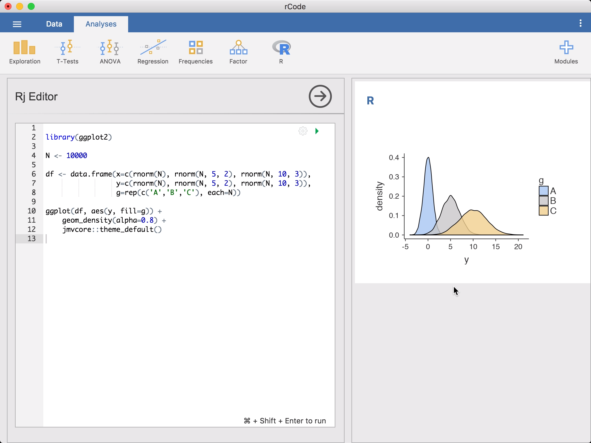
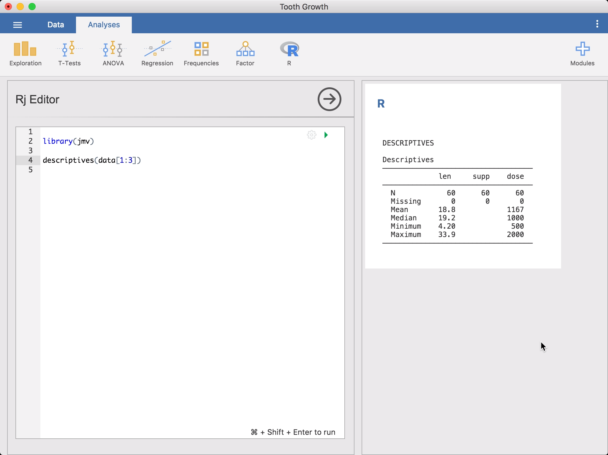
To run an R analysis, select Rj Editor from the R-icon in the Analyses ribbon. This will bring up the editor for entering your R code. The data set you have opened in jamovi is available to you as a data frame, simply as data. To get started, you might like to run descriptives on it.

Or if you prefer the dplyr approach, you could go:

library(jmv)
library(dplyr)
library(magrittr)

select(data, 1:3) %>% descriptives()

You’ll notice as you’re entering this code, Rj auto-suggests function names. To run the code, click on the green triangle or press Control + Shift + Enter (or ⌘ + Shift + Enter if you’re on a Mac). jamovi will run the R code and the results will appear in the results panel like other analyses. You can continue to make changes to the code, and then run it again.

By default, Rj makes use of the version of R bundled with jamovi. This includes many packages (jmv and all it’s dependencies), and will be sufficient for many people, but if you need to make use of additional R packages then you’ll need to make use of the System R version. If you select ⚙ (at the top right of the code box), you’ll see an option to change the R version used. The System R version uses the version of R you have installed on your system. This has the advantage that your R code now has access to all of the packages you have installed for that version of R. The last thing you will need is to have the jmvconnect R package installed in the R library on your system.

jmvconnect R package

The jmvconnect R package allows the R version on your system to access the data sets that you opened in jamovi. You can install it in R with:

install.packages('jmvconnect')

Once this is done, moving from the jamovi R to the System R should be seamless.

It’s worth remembering that sharing jamovi files with colleagues becomes a bit more complicated when you make use of the System R version. If they want to make changes and re-run your analyses, they will need to have the same R packages installed – that’s the price of flexibility!

When Rj runs R code, by default it makes the whole data set available as a data frame called data. However, it’s likely that your analysis only makes use of a few columns, and doesn’t need the whole data set. You can limit the columns made available to the analysis by including a special comment at the top of your script, of the form:

# (column1, column2, column3)

library(jmv)

...

In this instance, only the named columns will appear in the data data frame. This can speed the analysis up, particularly if you are working with large data sets. Additionally, this lets jamovi know that the analysis is only using these columns, and the analysis will not need to be re-run if changes are made to other columns.

There may be times where you’ll want to transition to an R session for analysing a data set. This is where the jmvconnect R package comes in handy. jmvconnect lets you read the data sets from a running jamovi instance into an R session. It has two functions: what() lists the available data sets, and read() reads them. For example, you might use:

> library(jmvconnect)
> what()

 Available Data Sets
 ─────────────────────────────────────
         Title           Rows    Cols
 ─────────────────────────────────────
    1    iris             150       5
    2    Tooth Growth      60       3
 ─────────────────────────────────────

and then read the data set with either of these two commands:

data <- read('Tooth Growth')
data <- read(2)

jmvReadWrite R package

The jmvReadWrite R package reads and writes jamovi-data-files (.omv) in R. It can be installed with:

install.packages('jmvReadWrite')

A typical use case would be if you wanted to process a large number of result files (e.g., CSV-files from several participants in an experiment or with responses from different questionnaires). Wrangling data is often easiest achieved in R. Once you have assembled your dataset from these files, you can write it using the write_omv()-function.

library(jmvReadWrite)

# assemble your data set (named dtaSet)...

write_omv(dtaSet, "FILENAME.omv")

Likewise does the read_omv-function permit you to read jamovi-data-files into R. Another typical use case would be reading a data file, doing manipulations that currently are not possible in jamovi, and then writing back the resulting modified file (in the jamovi file format).

library(jmvReadWrite)

dtaSet <- read_omv("FILENAME.omv")

# do some modifications to your data set

write_omv(dtaSet, "FILENAME.omv")

There is a couple of helper functions implemented in jmvReadWrite. They enable operations such as re-arranging the columns / variables of a data set (arrange_cols_omv), mass-converting a data files into the jamovi file format (convert_to_omv; e.g. from a statistics software that you used earlier), converting data files from long to wide format (long2wide_omv) and from wide to long format (wide2long_omv), adding variables from several data sets (merge_cols_omv), adding cases from several data sets (merge_rows_omv), or sort a data set after one or more variables (sort_omv).

Another possible use case for read_omv is the creation of R markdown files using the results of your jamovi analyses. The getSyn-parameter determines whether the syntax of the analyses contained in the file is extracted. For running the syntax, the jmv R package needs to be installed. If you would like to work with the results afterwards, it is recommended that you assign them to a variable (see the second eval below). Tables from the results can be converted into a data frame with the function asDF (e.g., result$main$asDF).

library(jmvReadWrite)
library(jmv)

data <- read_omv("FILENAME.omv", getSyn = TRUE)

# the analyses are stored in the attribute syntax
attr(data, "syntax")

# with using an index, the n-th analysis can be accessed (first line)
# and run / evaluated (second line)
attr(data, "syntax")[[1]]
eval(parse(text = attr(data, "syntax")[[1]]))

# often it is more useful to assign the results to a variable when
# running analyses and later on use the contents of that variable
eval(parse(text = paste0("result = ", attr(data, "syntax")[[2]])))
names(result)
# (returns the names of the output elements - tables, figures, and
# groups: sub-headings, e.g., Estimated Marginal Means in an ANOVA,
# that contain further tables and figures)